
| 일 | 월 | 화 | 수 | 목 | 금 | 토 |
|---|---|---|---|---|---|---|
| 1 | 2 | 3 | 4 | 5 | ||
| 6 | 7 | 8 | 9 | 10 | 11 | 12 |
| 13 | 14 | 15 | 16 | 17 | 18 | 19 |
| 20 | 21 | 22 | 23 | 24 | 25 | 26 |
| 27 | 28 | 29 | 30 |
- realtimerendering #highquality3d #fastrendering
- gaussianprojection #covariancematrix3d #anisotropicgaussians #ellipsoidalsplatting
- highfidelityreconstruction #sceneunderstanding #computationalgraphics
- 3dcontentcreation
- siggraphtechniques #aigraphics #3dmodelingalgorithms
- computervisionresearch #3dreconstructiontechniques #graphicsresearch
- 3dpointcloud #differentiablerendering #3dscenerepresentation #neuralrendering
- siggraph #3dsceneunderstanding #highquality3drendering #fastrendering
- gpuacceleration #aigraphics #virtualreality #augmentedreality #gamedevelopment
- anisotropickernels #ellipsoidalsplatting #orientedsplats #gradientbasedlearning
- pointbasedrendering #computergraphics #3dmodeling #volumerendering
- 3dsceneunderstanding #pointcloudrendering #neuralscenerepresentation
- gaussiansplatting #3dgaussiansplatting #pointbasedrendering
- advancedrenderingtechniques #neuralscenerepresentation
- splatrendering #3dpointcloud #differentiablerendering
- anisotropicgaussianlearning #gaussiansplatting #nonisotropicrenderinㅎ
- gaussiansplatting #3dgaussiancovariance #nerf #3dreconstruction
- nerf (neural radiance fields) #3dreconstruction #pointcloudrendering #volumerendering
- machinelearning3d #deeplearninggraphics #airendering
- differentiablerendering #machinelearning3d #deeplearninggraphics
- computergraphics #3dmodeling #virtualreality #augmentedreality #gamedevelopment
- turtlebot3 #터틀봇
- realtimerendering #machinelearning3d #deeplearninggraphics #computervision
- 3dscenerepresentation #covariancematrixoptimization #adaptivegaussians
- nextgengraphics #futureof3drendering #innovativerenderingtechniques
- optimizationalgorithms
- 3drenderingtools #pointcloudsoftware #3dvisualizationsoftware
- 3dscanning #digitaltwintechnology #3dcontentcreation
- geometrylearning #shapeoptimization #gpuacceleration #realtimerendering
- nerf (neural radiance fields) #3dreconstruction
- Today
- Total
Wiredwisdom
FAST DIFFERENTIABLE RASTERIZER FOR GAUSSIANS 본문
FAST DIFFERENTIABLE RASTERIZER FOR GAUSSIANS
Duke_Wisdom 2024. 6. 30. 21:04Our goals are to have fast overall rendering and fast sorting to allow approximate 𝛼-blending – including for anisotropic splats – and to avoid hard limits on the number of splats that can receive gradients that exist in previous work [Lassner and Zollhofer 2021]. To achieve these goals, we design a tile-based rasterizer for Gaussian splats inspired by recent software rasterization approaches [Lassner and Zollhofer 2021] to pre-sort primitives for an entire image at a time, avoiding the expense of sorting per pixel that hindered previous 𝛼-blending solutions [Kopanas et al. 2022, 2021].

Our fast rasterizer allows efficient backpropagation over an arbitrary number of blended Gaussians with low additional memory consumption, requiring only a constant overhead per pixel.
Constant Overhead
Low memory consumption
Efficiency back propagation
Our rasterization pipeline is fully differentiable, and given the projection to 2D (Sec. 4) can rasterize anisotropic splats similar to previous 2D splatting methods [Kopanas et al. 2021].
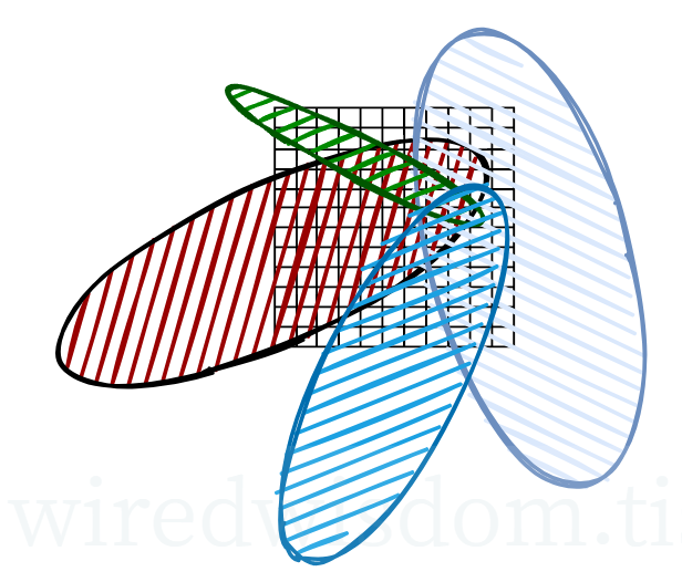
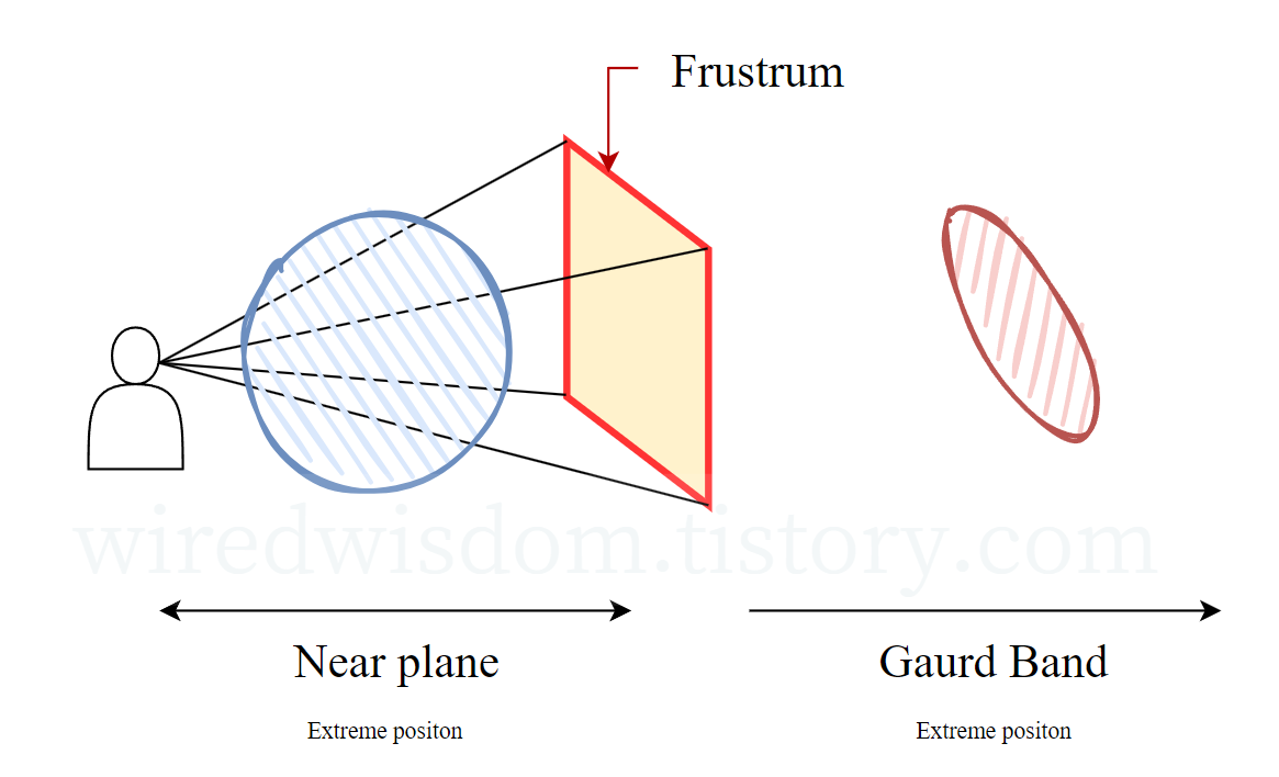
Our method starts by splitting the screen into 16×16 tiles, and then proceeds to cull 3D Gaussians against the view frustum and each tile.

Specifically, we only keep Gaussians with a 99% confidence interval intersecting the view frustum.

Additionally, we use a guard band to trivially reject Gaussians at extreme positions (i.e., those with means close to the near plane and far outside the view frustum), since computing their projected 2D covariance would be unstable.
We then instantiate each Gaussian according to the number of tiles they overlap and assign each instance a key that combines view space depth and tile ID.

We then sort Gaussians based on these keys using a single fast GPU Radix sort [Merrill and Grimshaw 2010].

Note that there is no additional per-pixel ordering of points, and blending is performed based on this initial sorting.

As a consequence, our 𝛼-blending can be approximate in some configurations. However, these approximations become negligible as splats approach the size of individual pixels.

We found that this choice greatly enhances training and rendering performance without producing visible artifacts in converged scenes. After sorting Gaussians, we produce a list for each tile by identifying the first and last depth-sorted entry that splats to a given tile.
No artifacts
Rendering performance

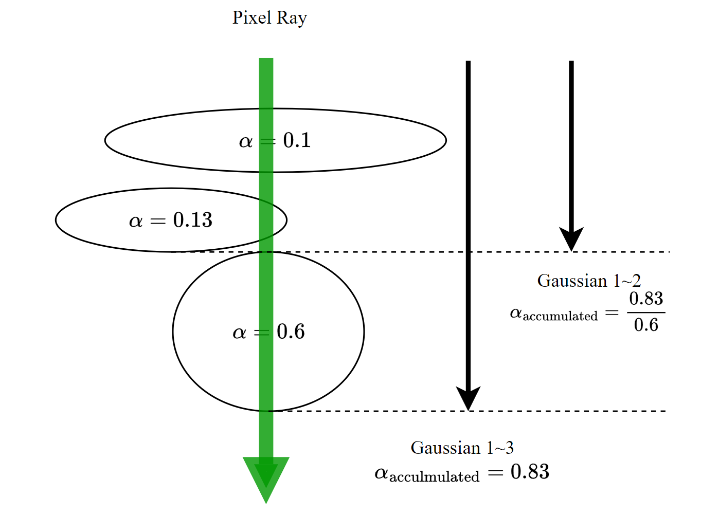
For rasterization, we launch one thread block for each tile. Each block first collaboratively loads packets of Gaussians into shared memory and then, for a given pixel, accumulates color and 𝛼 values by traversing the lists front-to-back, thus maximizing the gain in parallelism both for data loading/sharing and processing.

When we reach a target saturation of 𝛼 in a pixel, the corresponding thread stops. At regular intervals, threads in a tile are queried and the processing of the entire tile terminates when all pixels have saturated (i.e., 𝛼 goes to 1).
During rasterization, the saturation of 𝛼 is the only stopping criterion.

In contrast to previous work, we do not limit the number of blended primitives that receive gradient updates.
We enforce this property to allow our approach to handle scenes with an arbitrary, varying depth complexity and accurately learn them, without having to resort to scene-specific hyperparameter tuning.
Hyperparameter : 학습률(learning rate), 에폭(epoch) 수, 미니배치 크기(batch size), 레이어 수, 각 레이어의 뉴런
During the backward pass, we must therefore recover the full sequence of blended points per-pixel in the forward pass.
One solution would be to store arbitrarily long lists of blended points per-pixel in global memory [Kopanas et al. 2021].

To avoid the implied dynamic memory management overhead, we instead choose to traverse the per-tile lists again; we can reuse the sorted array of Gaussians and tile ranges from the forward pass.

To facilitate gradient computation, we now traverse them back-to-front.
The traversal starts from the last point that affected any pixel in the tile, and loading of points into shared memory again happens collaboratively. Additionally, each pixel will only start (expensive) overlap testing and processing of points if their depth is lower than or equal to the depth of the last point that contributed to its color during the forward pass. Computation of the gradients described in Sec. 4 requires the accumulated opacity values at each step during the original blending process. Rather than trasversing an explicit list of progressively shrinking opacities in the backward pass, we can recover these intermediate opacities by storing only the total accumulated opacity at the end of the forward pass. Specifically, each point stores the final accumulated opacity 𝛼 in the forward process; we divide this by each point’s 𝛼 in our back-to-front traversal to obtain the required coefficients for gradient computation.


'Vision > Gaussian Splatting' 카테고리의 다른 글
| 3D Gaussian's Split conditions (0) | 2024.07.04 |
|---|---|
| 3D Gaussian-Covariance (0) | 2024.07.03 |
| Convert 3D Gaussian to 2D splat Method (0) | 2024.06.22 |
| Overview (0) | 2024.06.22 |
| Ray for Final Color (Alpha-blending & NeRF) (0) | 2024.06.22 |


